admix_display.html

How to display admixture coefficients (Q matrix) spatially?

Displaying admixture coefficients is important in order to interpret the outputs of TESS or STRUCTURE, and generally to understand the genetic structure of a population in geographic space. Like STRUCTURE, TESS displays the admixture coefficients in a bar chart format available from the GUI and stored as a PNG image in the TESS working directory. Better representations of this bar chart image can be obtained using DISTRUCT or R (barplot command). The textual outputs of TESS are actually stored in the CLUMPP POPFILE format, which can be used as direct input to the DISTRUCT program after a simple cut-and-paste operation.

Many users agree that the one-dimensional bar chat representation is unsatisfactory when data are two-dimensional. Here we provide an R script that generates two-dimensional representations of admixture levels. Note that the hard-clustering colored tessellation displayed by TESS is a no-admixture display of individual membership, each color representing a cluster. In this page, we propose to use the graphical library of the statistical software R to display spatial interpolates of the admixture coefficients (Q matrix) in two dimensions.

Let's show an illustration of the use of our script. We simulated 647 diploid individuals genotyped at 50 microsatellite loci, using a realistic model of spatial range expansion through Europe. The example data set is available by clicking this link (one individual = one row). The spatial coordinates were recorded as longitude and latitude. The admixture coefficients were computed using CLUMPP, but any output from TESS or STRUCTURE is also acceptable. We used Kmax = 6 clusters, but only K=3 were associated with significant values of admixture levels. The admixture coefficients are shown in the figures below

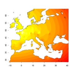
admixture level in cluster 1

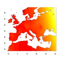
admixture level in cluster 2

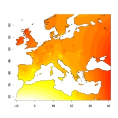
admixture level in cluster 3

Here we make available the R code (distributed with no warranty) which enabled us to compute these interpolated map using the Kriging method. To replicate the figures on your computer (independent on your OS) follow the next instructions

Download R from the CRAN website
Create a working folder
Place your two files "mydata.coord" (spatial coordinates in longitude deg N and latitude deg E) and "outfile.txt" (Q matrix) in the working folder.
Launch R and change the R working directory (should be the same as your working folder)
Install the R package 'maps' and 'fields' (from a remote R server)
Place the file "plot.admixture.r" into the working folder
Type 'source("plot.admixture.r")' from the R command line.

The basic R command called in this script is the tessplot function which can be also be invoked with the following arguments:

tessplot(tessfile = "mydata.coord", qmatrix = "outfile.txt", clustermap = 1, colpalette = colrp, mapadd = T)

tessplot(tessfile = "mydata.coord", qmatrix = "outfile.txt", clustermap = 1, colpalette = colrp, mapadd = T)

tessfile: A matrix in the TESS format or a matrix of geographic coordinates (Longitude, Latitude) for each individual.

qmatrix: a matrix of ancestry coefficients from TESS, STRUCTURE or CLUMPP (see for example "outfile.txt").

clustermap: An integer value for which cluster map is displayed.

colpalette: A color palette, see the examples below.

mapadd: Logical. If TRUE, a world map is added.

par(mfrow = c(1,3))

colrp = colorRampPalette(c("white","blue", "darkblue"))(20)
tessplot(cluster = 1, colp = colrp)

colrp = colorRampPalette(c("white","yellow", "orange"))(20)
tessplot(cluster = 2, colp = colrp)

colrp = colorRampPalette(c("white","green", "green4"))(20)
tessplot(cluster = 6, colp = colrp)

Do not hesitate to send e.mails!